Deep Learning: What Is Regularisation ?
Categories and Comparison of Regularization Methods
1. What is Regularization
(Source: Gpt-4o mini)
Regularization is a technique to prevent overfitting, mainly used in machine learning and statistical modeling. Overfitting happens when a model learns the training data too well, capturing noise instead of underlying patterns, resulting in poor performance on new data.
Core idea of regularization:
- Penalize complex models: Add an extra penalty term (regularization term) to the loss function to constrain model complexity. This encourages optimization to consider both prediction accuracy and model simplicity.
Benefits of regularization:
- Improve generalization: Reduce model complexity to achieve more stable performance on unseen data.
- Feature selection: L1 regularization can set some feature weights to zero.
- Control overfitting: Prevent the model from learning noise in training data, improving predictive ability.
2. Why Regularize
(My notes)
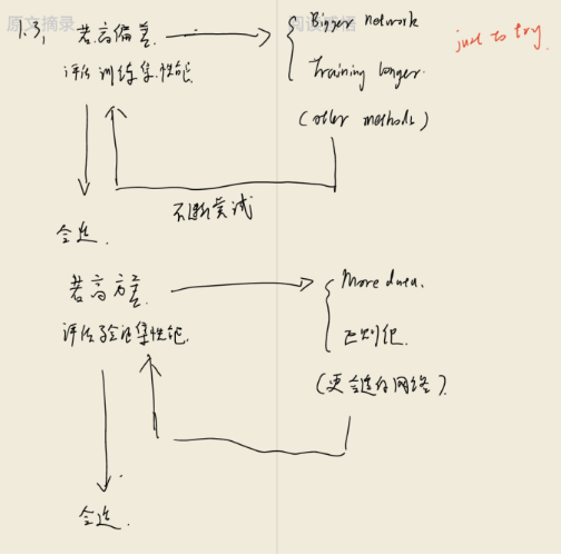
- Training a model is a long and iterative process. When fitting data, we usually encounter: overfitting, underfitting, and just-right fitting—corresponding to high variance, high bias, and ideal fit.
- To reduce high variance (overfitting), three common approaches exist:
- Clean the data (time-consuming)
- Reduce model parameters and complexity
- Add a penalty factor, i.e., regularization
For a regression model:
Higher-order terms make the model more flexible, increasing variance. Limiting these coefficients (e.g., $\theta_3, \theta_4$) helps reduce overfitting:
3. How to Regularize Models
- Introduce three common methods:
- $L_2$ Regularization
- $L_1$ Regularization
- Dropout
3.1 $L_2$ Parameter Regularization (Frobenius Norm)
Also known as Ridge Regression or Tikhonov Regularization.
-
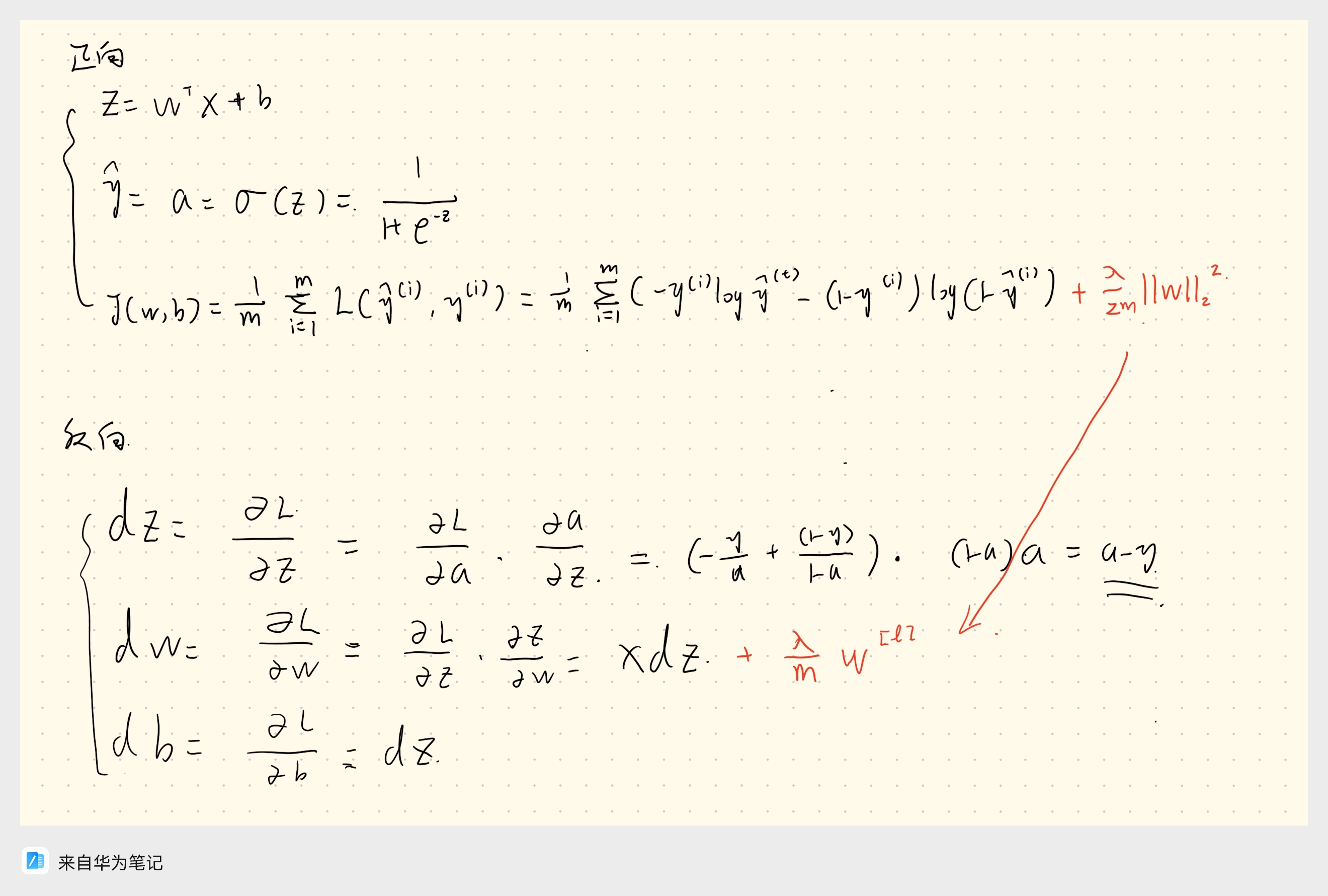
Method: Add a regularization term to the objective function:
-
For logistic regression:
-
$\mathbf{w} = [w_1, w_2, …, w_n]$ is the weight vector (excluding bias). The regularization term penalizes large weights to prevent overfitting.
-
$||\mathbf{w}||_2^2 = w_1^2 + w_2^2 + … + w_n^2$
-
$\frac{\lambda}{2m}$ scales the regularization effect relative to dataset size.
Why $L_2$ works:
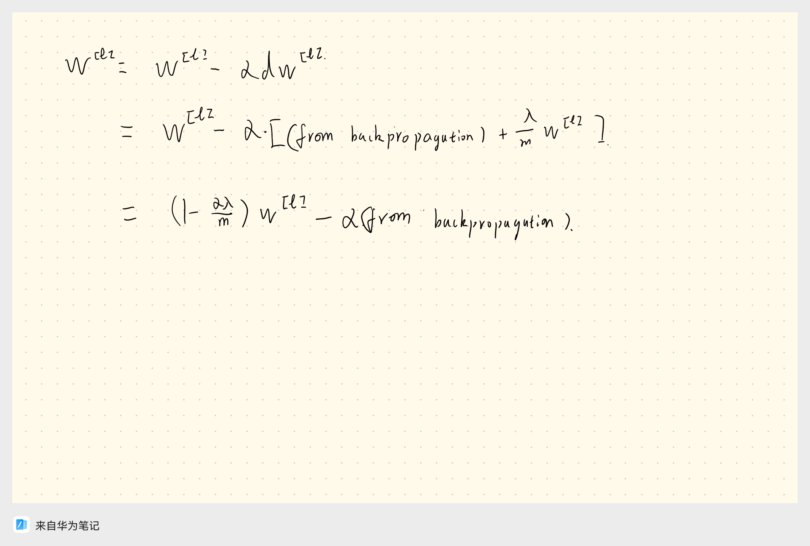
- Adds $\Omega(\theta) = \frac{1}{2m} ||\mathbf{w}||_2^2$ to the loss, affecting backpropagation.
- Weight update effectively performs weight decay, shrinking all weights proportionally.
3.2 $L_1$ Regularization
- In linear regression, called Lasso Regression:
- Sparsity: Many parameters become zero, achieving feature selection—important in high-dimensional tasks like NLP or genomics.
- L1 can also reduce overfitting, though its primary use is sparsity.
Reference: Deep Understanding of L1/L2 Regularization
3.3 Dropout (Random Deactivation)
- Common in CV and deep learning.
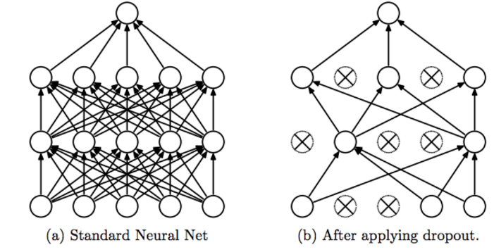
- Randomly remove neurons during training to reduce overfitting.
- Inverted Dropout: scale activations by keep probability to maintain expected value:
d3 = np.random.rand(a3.shape[0], a3.shape[1]) < keep_prop
a3 = a3 * d3
a3 /= keep_prop